

Econometric mannequin
DID mannequin
Authorities intervention is measured by fiscal expenditure and the coverage orientation of establishing new power demonstration cities. Right here, we studied the influence of presidency intervention and industrial construction on EE. As DID can clear up endogenous issues generally confronted within the present literature26, the development of recent power demonstration cities may be seen as a “pure experiment”. On this examine, fiscal expenditure, coverage orientation, and industrial construction had been thought-about as core explanatory variables and a DID mannequin was constructed to estimate the impact of presidency intervention and monetary expenditure on EE. The equation for this mannequin is as follows:
$$LnY_{it} = beta_{0} + beta_{1} du_{it} + beta_{2} dt_{it} + beta_{3} du_{it} occasions dt_{it} + lambda_{{1}} LnFE_{it} { + }lambda_{{2}} LnIND_{it} { + }lambda_{{textual content{n}}} LnX_{it} + T_{{textual content{t}}} + mu_{i} + varepsilon_{it}$$
(1)
the place, (i) and (t) are cities and years, respectively; the defined variable (Y_{it}) is the annual EE of every metropolis, (du_{it}) is a area dummy variable, and (dt_{it}) represents the time dummy variable. The interplay coefficient (beta_{3}) displays the web impact of coverage orientation on EE. (FE_{it}) is fiscal expenditure, (IND_{it}) is industrial construction, (X_{it}) is the management variable matrix, comprising financial growth degree, urbanisation degree, overseas funding and expertise degree. (T_{t}) is the time-fixed impact, (mu_{i}) is the individual-fixed impact, and (varepsilon_{it}) is the random disturbance time period. Logarithmic processing was carried out on the information of variables to cut back the affect of skewness and heteroscedasticity.
Spatial econometric mannequin
A sure spatial correlation was noticed as a result of cities will not be unbiased. Fiscal expenditure, coverage orientation, and industrial construction have an effect on regional EE and may additionally influence adjoining areas. Thus, on this examine, spatial elements had been included into the mannequin, taking authorities intervention and industrial construction as core explanatory variables. The spatial econometric mannequin is as follows.
$$start{gathered} L{textual content{n}}EE_{it} = alpha_{0} + rho WLnEE_{it} + beta_{1} du_{it} occasions dt_{it} + beta_{2} LnFE_{it} + beta_{3} LnIND_{it} + beta_{n} LnX_{it} + hfill , xi_{1} Wdu_{it} occasions dt_{it} + xi_{2} WLnFE_{it} + xi_{3} WLnIND_{it} + xi_{n} WLnX_{it} + T_{t} + mu_{i} + varepsilon_{it} hfill varepsilon_{it} = gamma varepsilon_{it} + nu_{it} hfill finish{gathered}$$
(2)
the place (W) is the geospatial distance weight, (WLnEE_{it}) is the spatial lag of the defined variable, (rho) and (xi) are the space-effect coefficients. (nu_{it}) is the error time period of (varepsilon_{it}). When (rho { = }xi { = 0}), it degenerates right into a spatial error mannequin (SEM). When (xi { = }gamma { = 0}), it degenerates right into a spatial lag mannequin (SLM). When (gamma { = 0}), it’s the SDM.
Samples and information
On this examine, 3540 balanced panel observations of 236 cities in China from 2005 to 2019 had been used to research the influence of fiscal expenditure, new power demonstration metropolis building coverage orientation, and industrial construction on EE. The investigation of the development coverage orientation of recent power demonstration cities solely thought-about the primary batch of demonstration cities, and information samples on the prefecture-level had been used. To make sure the robustness of the conclusion, county-level cities, districts (autonomous prefectures), and industrial park cities had been eradicated from the primary batch of demonstration cities established in 2014. Subsequently, 47 and 189 cities had been generated within the experimental and management teams, respectively. To research its regional characters, the 30 provinces in China had been divided into japanese, central and western regional in keeping with geographic location. Particularly, the japanese area consists of 12 provinces and cities, particularly Beijing, Hebei, Tianjin, Shandong, Jiangsu, Shanghai, Zhejiang, Fujian, Guangdong, Hainan, Liaoning and Guangxi; The central area consists of the 9 provinces of Shanxi, Henan, Hubei, Hunan, Anhui, Jiangxi, Internal Mongolia, Heilongjiang and Jilin; The western area covers 9 provinces, particularly Chongqing, Sichuan, Shaanxi, Yunnan, Guizhou, Gansu, Qinghai, Ningxia and Xinjiang. Above 236 cities had been divided into three areas primarily based on their belong provinces. The information used on this examine had been obtained from the statistical yearbook of cities in any respect ranges, the China Metropolis Statistical Yearbook, and the Statistical Bulletin of Social and Financial Growth. The lacking values had been uniformly crammed by interpolation.
Variable description
Interpreted variables
The course distance operate (DDF) proposed by Chung et al.27 is extensively utilized in power and environmental effectivity. Nonetheless, a limitation of utilizing the DDF is that every one the enter and output components should change in the identical course. Zhou et al.28 additional proposed the NDDF, which might successfully clear up the issue of enter and output elements altering in the identical course. Subsequently, within the current examine, the NDDF was used to measure EE. The NDDF is outlined as follows28:
$$overrightarrow {D} (x,y,b;g) = sup left{ {W^{T} beta :((x,y,b){ + }g occasions diag(beta )) in T} proper}$$
the place (g = ( – g_{x} ,g_{y} , – g_{b} )) represents the required course vector, (W = (W_{x} ,W_{y} ,W_{b} )) represents the weighting vector of every enter–output factor, and (beta = (beta_{x} ,beta_{y} ,beta_{b} )^{T} ge 0) represents the variable proportion of every enter and output issue.
Vitality (E), capital (Ok), and labour (L) had been taken as enter elements. The gross home product (GDP) of every metropolis (G) is taken as fascinating output. Sulphur dioxide (S), smoke (mud) emissions (C), and wastewater discharge (P) had been undesirable outputs in every city2. Utilizing NDDF, the DEA mannequin of EE of 236 cities was constructed as follows:
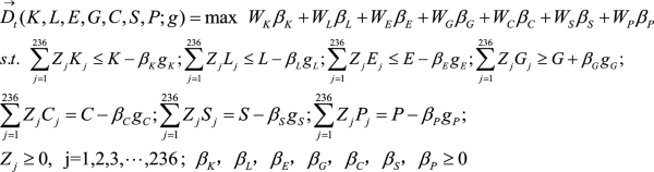
(3)
the place the course vector (g = ( – Ok, – L, – E, + G, – C, – S, – P)), referring to the analysis of Liu et al.29, the burden matrix (W^{T} = left( {frac{1}{9},frac{1}{9},frac{1}{9},frac{1}{3},frac{1}{9},frac{1}{9},frac{1}{9}} proper)) is given, substituting into Eq. (3), and acquiring (beta_{j}^{ * } = (beta_{jK}^{ * } ,beta_{jL}^{ * } ,beta_{jE}^{ * } ,beta_{jG}^{ * } ,beta_{jC}^{ * } ,beta_{jS}^{ * } ,beta_{jP}^{ * } )) by way of linear programming, that’s, the optimum answer of the slack variable of the (j)th metropolis. The EE for every metropolis within the corresponding yr is calculated as follows:
$$start{aligned} EE_{j} = & frac{1}{6}left[ begin{gathered} frac{{G_{j} /K_{j} }}{{(G_{j} + beta_{jG}^{ * } G_{j} )/(K_{j} – beta_{jK}^{ * } K_{j} )}} + frac{{G_{j} /L_{j} }}{{(G_{j} + beta_{jG}^{ * } G_{j} )/(L_{j} – beta_{jL}^{ * } L_{j} )}} hfill + frac{{G_{j} /E_{j} }}{{(G_{j} + beta_{jG}^{ * } G_{j} )/(E_{j} – beta_{jE}^{ * } E_{j} )}} + frac{{G_{j} /C_{j} }}{{(G_{j} + beta_{jG}^{ * } G_{j} )/(C_{j} – beta_{jC}^{ * } C_{j} )}} hfill + frac{{G_{j} /S_{j} }}{{(G_{j} + beta_{jG}^{ * } G_{j} )/(S_{j} – beta_{jS}^{ * } S_{j} )}} + frac{{G_{j} /P_{j} }}{{(G_{j} + beta_{jG}^{ * } G_{j} )/(P_{j} – beta_{jP}^{ * } P_{j} )}} hfill end{gathered} right] { = } & frac{1}{6}left[ {frac{{(1 – beta_{jK}^{ * } ) + (1 – beta_{jL}^{ * } ) + (1 – beta_{jE}^{ * } ) + (1 – beta_{jC}^{ * } ) + (1 – beta_{jS}^{ * } ) + (1 – beta_{jP}^{ * } )}}{{1 + beta_{jG}^{ * } }}} right] { = } & frac{{1 – frac{1}{6}(beta_{jK}^{ * } + beta_{jL}^{ * } + beta_{jE}^{ * } + beta_{jC}^{ * } + beta_{jS}^{ * } + beta_{jP}^{ * } )}}{{1 + beta_{jG}^{ * } }},j = 1,2,3, ldots {,236} finish{aligned}$$
(4)
In measuring EE, the labour drive (L) of every metropolis was measured primarily based on the variety of staff. Owing to the shortage of city-scale power consumption information within the statistical yearbook, provincial power consumption information had been retrieved for every metropolis in keeping with the sunshine information worth utilizing a linear mannequin with out intercept30. The quantity of capital funding was estimated utilizing the perpetual stock method31. The GDP of every metropolis was used to precise the fascinating outputs. Sulphur dioxide (S), wastewater discharge (P), and smoke (mud) emissions (C) had been estimated utilizing information on industrial sulphur dioxide emissions, industrial wastewater discharges, and industrial smoke and dirt emissions2. On this examine, the influence of value elements on analysis was diminished by adjusting all value information in 2005.
Core explanatory variables
(1)
Coverage orientation ((du occasions dt)) The coverage orientation investigated on this article is the brand new power demonstration metropolis pilot dummy variable, (du occasions dt), the place (du) is the processing variable, indicating whether or not town was chosen as the primary batch of demonstration cities in 2014; if chosen, (du{ = 1}), in any other case (du{ = 0}). Moreover, (dt) is a time dummy variable; (dt{ = 0}) earlier than the pilot metropolis was chosen, and (dt{ = 1}) was chosen after the choice.
(2)
Fiscal expenditure Fiscal expenditure is a authorities macroeconomic management measure that may intervene in financial growth, air pollution and carbon emission reductions, and useful resource allocation. By investing in new power business infrastructure and technological innovation, the federal government can constantly enhance the technological innovation atmosphere and technological service services, guiding the movement of modern sources and attracting extra enterprises and analysis establishments to extend their funding. Rising funding within the new power business will speed up the event and utilisation of recent power, cut back pollutant emissions, and promote the development of EE. On this examine, the extent of city monetary expenditure was measured because the proportion of city common monetary price range expenditure to GDP.
(3)
Industrial construction The continual adjustment of the economic construction can promote the rational allocation of useful resource components in varied industries and preserve a steadiness between enter and output. The Thiel index is a vital indicator for measuring the affordable allocation of commercial useful resource components in cities. On this examine, the Thiel index was used to measure the economic construction. As described in Gao et al.32, the calculation is carried out as follows:
$$frac{{1}}{IND}{ = }sumlimits_{{}}^{{}} {left( {frac{{Y_{{textual content{i}}} }}{Y}} proper)} ln left( {frac{{Y_{i} }}{{L_{i} }}/frac{Y}{L}} proper)$$
the place (Y_{i}) and (Y) signify the added worth and GDP of the three industries, respectively; (L_{i}) and (L) are the employment and complete employment of the three industries. The (IND) worth displays an inexpensive diploma of commercial construction. The bigger the worth, the extra affordable the allocation of sources and manufacturing elements amongst sectors.
Management variables
The financial growth degree (PGDP) was expressed in GDP per capita. International direct funding (FDI) is measured because the proportion of FDI utilised by every metropolis in regional GDP33. Urbanisation degree (URBAN) was measured because the ratio of the city inhabitants to the full inhabitants. Technological innovation (TI) is measured because the proportion of staff engaged in scientific analysis, technical providers, and geological prospecting to these employed within the unit on the finish of the yr. To get rid of heteroscedasticity, logarithmic processing was carried out for every variable. The descriptive statistical evaluation of every variable is introduced in Desk 1.


