
SkS Analogy 9 – The greenhouse impact is a stack of blankets
Posted on 12 July 2023 by Evan, Bob Loblaw, jg
This can be a second revision of a earlier analogy. It provides an appendix with a mathematical mannequin of the water tank instance. The earlier revision is right here. The unique model is right here.
Tag Line
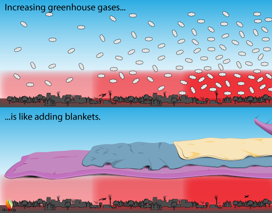
The greenhouse impact is sort of a stack of blankets on a winter night time.
Elevator Assertion
Extra blankets = extra heat: The greenhouse impact is like blankets warming the Earth. Whether it is 10°C (50°F) in your bed room, you want a couple of blankets to maintain your self heat. Extra blankets = extra warming. Too many blankets and also you sweat. The greenhouse impact is an effective factor, up to a degree.
Local weather Science
For the atmospheric temperature to be steady (i.e., no international warming nor cooling), the Earth should lose simply as a lot power to house because it features from the solar. How does this work? If international warming is going on, what is going to ever permit it to cease and for atmospheric temperatures to cease rising?
The solar sends us extra power that we are able to use, within the type of a broad spectrum of sunshine. Earth absorbs about 70% of the incident mild, and displays the remainder out to house. The 70% of the suns power that’s absorbed heats the Earth. Though the power that comes from the solar is within the type of a broad spectrum of wavelengths, issues on Earth predominantly re-emit infrared radiation. Infrared radiation is emitted in all instructions, together with skyward. If you end up sitting subsequent to a fireplace, you’re feeling the infrared warmth from the fireplace, and a few of that infrared warmth strikes upward, in the direction of house. Does it make it to house?
There are lots of issues which will stop infrared radiation from making it to house: a passing airplane might take in some, clouds, and a few gases within the ambiance are notably efficient at capturing infrared radiation: the so-called greenhouse gases (GHG’s). The extra GHG’s we pump into the ambiance, the extra infrared radiation it traps, and the extra the ambiance heats up. That is international warming. But when the ambiance warms up after we add extra GHG’s, what limits the quantity of warming?
When issues warmth up they emit extra infrared radiation. Evaluate the warmth emitted from a smoldering fireplace to that from a roaring fireplace. Because the ambiance warms up, it emits extra infrared radiation, a few of it skyward. The hotter the ambiance, the extra infrared radiation is emitted. Though GHG’s inhibit the movement of infrared radiation by means of the ambiance, a hotter ambiance forces extra infrared radiation up and out into house. Finally a steadiness is reached the place a hotter ambiance manages to pressure sufficient infrared radiation up and out into house to reject to house the identical quantity of photo voltaic power absorbed by the Earth.
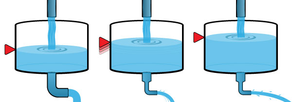
To visualise how this works, think about a tank, with water flowing out and in. The water degree is balanced when the circulation fee into the tank equals the circulation fee out of the tank. What occurs if we prohibit the outflow (center image above)? That is corresponding to how GHG’s prohibit the circulation of infrared radiation by means of the ambiance. Initially the outflow fee decreases, inflicting much less water to circulation out than into the tank. The water degree rises in response. That is corresponding to atmospheric temperature growing. However a better water degree applies extra strain to the outlet, growing the outflow fee. As the extent of water rises within the tank, the outlet circulation fee will increase, till a brand new steadiness is reached between influx and outflow. The results of the restriction on the outlet is a better water degree within the tank, however in any other case the influx and outflow charges are the identical as firstly.
Though a few of the particulars right here might sound sophisticated and trigger head scratching, the essential idea is straightforward: including GHG’s to the ambiance is like including extra insulating blankets on high of you: you get hotter.
Historic Perspective
Replete with fancy graphics, high-tech movies, and communicated throughout social-media channels, it usually feels as if local weather science is a product of our trendy age: the factor driving GHG emissions. However crack open a dusty journal from days passed by, and we quickly understand that our data concerning the “warming blankets” over Earth dates again to the daybreak of the Industrial Revolution.
In 1858 a feminine American researcher, Eunice Foote, printed the next in The American Journal of Science and Arts (Vol XXII, Nov. 1856)
“The very best impact of the solar’s rays I’ve discovered to be in carbonic acid gasoline [CO2]. … An ambiance of that gasoline would give to our earth a excessive temperature; and if as some suppose, at one interval of its historical past, the air had combined with it a bigger proportion than at current, an elevated temperature from its personal motion, in addition to from elevated weight, should have essentially resulted.”
5 years later John Tyndall, the particular person usually acknowledged as discovering the heat-trapping traits of CO2 and different GHG’s, wrote the next within the Philosophical Transactions of the Royal Society of London (Vol. 151 (1861), pp. 1-36)
“Now if, because the above experiments point out, the chief affect be exercised by the aqueous vapour, each variation of this constituent should produce a change of local weather. Comparable remarks would apply to the carbonic acid [CO2] subtle by means of the air; whereas an virtually inappreciable admixture of any of the hydrocarbon vapours would produce nice results on the terrestrial rays and produce corresponding modifications of local weather.”
We have identified for a really very long time concerning the heat-trapping impact of GHG’s and that they act like a pile of blankets over the Earth.
Appendix (added July 2023)
The water tank instance is a “descriptive mannequin”. Utilizing plain phrases and a determine, it visualizes a leaky water tank and the way the water degree responds when the circulation fee out the underside is decreased. The water tank instance may also be expressed quantitatively with a mathematical mannequin. Such fashions are helpful for visualizing the habits of the water tank with graphs
Changing a verbal description right into a mathematical mannequin is completed by describing the circulation into/out of the tank utilizing a collection of equations. We translate the day-to-day language of the descriptive mannequin into the language of arithmetic. The web impact of those circulation equations additionally tells us concerning the peak of the liquid within the tank.
The primary equation describes the water circulation into the highest of the tank. Let’s set this at a relentless fee of 400 (with models of quantity per unit time).
Influx = 400
The second equation is the strain pushing water out of the drain on the backside. That is zero when the bucket is empty, and will increase proportional to the depth of water within the tank. This can be a linear relationship, the place the multiplier a (associated to the liquid’s density) turns peak into strain:
Strain at drain = a*(water degree)
To translate influx into water depth, we’d like the tank space. Let’s make it 400 (models of space), in order that the fixed influx of 400 would make the extent rise by 1 peak unit over one time period.
We additionally want to find out the outflow fee by means of the drain. We’d like the strain (above), and the realm of the drain, and a few fluid dynamics associated to how simply the liquid flows by means of the drain. Let’s preserve it easy and assume that the multiplier a and the drain traits all work out in order that the outflow might be given by:
outflow = (space of drain)* (water degree)
…we are able to mix these into our full mannequin:
(influx – outflow)/(space of bucket) = (change in water degree)
…or, by substituting the earlier equations
(400 – space of drain * water degree)/400 = change in water degree
However how can we flip this right into a graph (or set of numbers) that reveals the change in water degree over time? Like several journey of a thousand miles, start with a single step. And comply with that with one other step. And one other. And our steps will likely be steps in time.
Let’s begin with an empty tank, and a drain with an space of two.
1. In step one, we add 400 from our influx. The tank is initially empty, so outflow is initially zero. The influx will enhance the water degree within the tank to 1.
2. Within the second step, our influx is once more 400, however our outflow is now 2*1=2 (drain space occasions water degree), so the online enter is barely 398, The extent rises by 0.995, to 1.995.
3. At step 3, influx continues to be 400, outflow is now 2*1.995=3.99, and the water degree rises to 2.985.
…and so forth.
At time 1000, our water degree has risen to 198.7, We nonetheless have an enter of 400, however our outflow by means of the drain is 397.3. The web enter is barely 2.7, and the water degree is rising very slowly. We have reached a nearly-constant water degree.
So, now what occurs if we partially shut the drain at time 1000? Let’s scale back its space from 2 to 1.
The speedy impact is to scale back the outflow by half, to about 198.7
Now the online enter jumps from 2.7 to 201.3 (400 – 198.7).
…and the water degree begins to rise rapidly once more.
..and we preserve calculating new time steps transferring ahead with the brand new drain space, till issues stabilize.
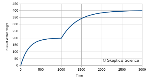
We are able to put this mannequin right into a spreadsheet, the place every row represents an extra step in time, and generate the next graphs. First, the water degree versus time:
After which the circulation charges:
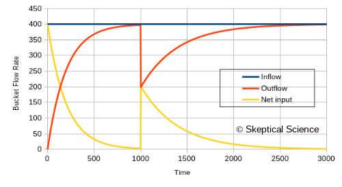
…and now now we have one other visible of how decreasing the circulation out of the underside of the water tank results in an increase within the water degree. The numbers are additionally intuitive:
To compensate for an influx of 400, we’d like an outflow of 400.
The water degree rises till the strain is excessive sufficient for the drain to permit an outflow of 400.
After we prohibit the drain measurement at time 1000, decreasing it by one half, the outflow drops by half.
The water degree must rise to twice the peak (twice the strain) to extend the outflow to 400 once more.
If we return to our equations, the place our mathematical mannequin is (400 – space of drain * water degree)/400 = change in water degree
The change in water degree is zero when now we have a drain space of two and a water degree of 200, or if now we have a drain space of 1 and a water degree of 400.
…however the step-by-step mannequin additionally reveals us how we get there.
Now you will have seen how a descriptive mannequin might be translated right into a mathematical mannequin.
If you wish to play with this mannequin, Skeptical Science has supplied a CSV file at this hyperlink. It may be imported into any spreadsheet program, and provides you with the equations wanted to generate the information. You will want to create your personal graphs, although – that may’t be saved in a CSV file.
After you have this in a spreadsheet, you’ll be able to change the values for the fixed influx, the preliminary water degree, the realm of the tank, the preliminary and remaining space of the drain (and the time at which the change happens), and the scale of the time step. You may discover the mannequin to see the way it behaves beneath totally different circumstances – what it the water degree begins at 400? what if the drain measurement begins at 1 and alter to 2? and so on.
We have now deliberately prevented models on this mathematical mannequin. It doesn’t matter what size models or time models you utilize, so long as you’re constant. Size in cm, mm, m, inches, toes, or furlongs. Space in the identical unit2, and quantity in the identical unit3. Time might be seconds, minutes, hours, and so on. Custom dictates that if you choose furlongs for size, that you simply use fortnights for time.


