
EMSs will be partitioned into three predominant strategies: optimization-based strategies, rule-based strategies, or extra lately, learning-based strategies, as depicted in Fig. 4.
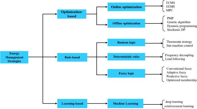
Classification of EMS of HPS.
The instructed EMS
The instructed EMS goals to regulate the motor velocity successfully and stabilize the voltage of the DC bus. Oblique Discipline Oriented Management (IFOC) is used to regulate the motor velocity. This technique gives the d-q voltage references for the State House Vector PWM (SVPWM) system. Hybridization between the differential flatness idea and metaheuristic optimization is used to regulate the bus voltage optimally.
SynRM drive IFOC design
The SynRM’s Oblique Discipline Oriented Management (IFOC), as proven in Fig. 5, contains three management loops: an exterior velocity management loop, an inside present management loop for ({i}_{sd}) and one other loop for ({i}_{sq}). The primary loop output generates the quadrature reference present, which is in comparison with the present worth ensuing from the present measurements. Their error is utilized to the enter of the isq present controller. Equally, there’s a present regulation loop of direct present isd. The outputs of the 2 inside loops isq and isd are utilized to a decoupling block producing the reference voltages ({v}_{sd}^{ref}) and ({v}_{sq}^{ref}). By passing from the reference (d-q) to the reference (α,β), the 2 voltages reference ({v}_{salpha }^{ref}), ({v}_{sbeta }^{ref}) required by the House Vector Modulation (SVM) block.
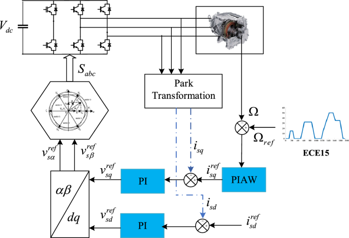
Diagram of SynRM Discipline-oriented management.
The proposed optimum differential flatness-based EMS
The proposed EMS is predicated on optimum differential flatness. It’s divided into two elements: a lower-level controller and a higher-level controller. The upper-level controller generates the ability reference for every supply. The ability references created by the inverse dynamic in Eq. (16) and Eq. (18) are divided by the measured supercapacitor and battery voltages to generate the reference currents for the supercapacitor and battery converters. The lower-level controller adjusts for DC-bus present variations and compensates for the DC-bus present harmonics utilizing a supercapacitor, which leads to improved power high quality and battery lifecycle enhancement. Determine 6, illustrates the operational management construction.
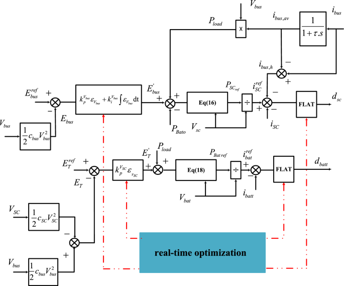
Proposed optimum differential flatness-based EMS.
Vitality regulation
Within the thought-about HPS, the flat mannequin is expressed by its flat output (y={[{y}_{1} {y}_{2}]}^{T}), management variable (u={[{u}_{1} {u}_{2}]}^{T}), and state variable (x={[{x}_{1} {x}_{2}]}^{T}),
The place:
$$y = left[ {begin{array}{*{20}c} {E_{Bus} } {E_{T} } end{array} } right],u = left[ {begin{array}{*{20}c} {P_{SC}^{ref} } {P_{Bat}^{ref} } end{array} } right],x = left[ {begin{array}{*{20}c} {V_{bus} } {V_{SC} } end{array} } right]$$
(13)
From Eq. (2), the state variable ({x}_{1}) representing Vbus will be expressed as follows:
$$x_{1} = left( {{raise0.7exhbox{${2y_{1} }$} !mathord{left/ {vphantom {{2y_{1} } {c_{bus} }}}proper.kern-0pt} !lower0.7exhbox{${c_{bus} }$}}} proper),^{{{raise0.7exhbox{$1$} !mathord{left/ {vphantom {1 2}}proper.kern-0pt} !lower0.7exhbox{$2$}}}} = lambda_{1} (y_{1} )$$
(14)
From Eq. (4), the state variable ({x}_{2}) representing VSC will be expressed as follows:
$$x_{2} = left( {{raise0.7exhbox{${2(y_{2} – y_{1} )}$} !mathord{left/ {vphantom {{2(y_{2} – y_{1} )} {c_{SC} }}}proper.kern-0pt} !lower0.7exhbox{${c_{SC} }$}}} proper)^{{{raise0.7exhbox{$1$} !mathord{left/ {vphantom {1 2}}proper.kern-0pt} !lower0.7exhbox{$2$}}}} = lambda_{2} (y_{1} ,y_{2} )$$
(15)
The SC energy reference PSCref, thought-about the primary enter management variable, ({u}_{1}), is derived from Eqs. 5, 7, and 9.
$$u_{1} = 2P_{SC,max } left[ {1 – left( {1 – frac{{dot{y}_{1} + sqrt {frac{{2y_{1} }}{{c_{bus} }},} ,i_{Load} – P_{Bato} }}{{P_{SC,max } }}} right)^{{{raise0.7exhbox{$1$} !mathord{left/ {vphantom {1 2}}right.kern-0pt} !lower0.7exhbox{$2$}}}} } right] = vartheta_{1} (y_{1} ,dot{y}_{1} ) = P_{{SC_{ref} }}$$
(16)
with PSCmax is the SC converter’s most energy restrict. It may be outlined as
$$P_{SC,max } = V_{SC}^{2} /4r_{SC}$$
(17)
In regards to the second enter, the ability reference of the battery PBattref is calculated from Eqs. 5, 6, and 9 as follows:
$$u_{2} = 2P_{Bat,,max } left[ {1 – left( {1 – frac{{dot{y}_{2} + sqrt {frac{{2y_{1} }}{{c_{bus} }},} ,i_{Load} }}{{P_{,Bat,,max } }}} right)^{{{raise0.7exhbox{$1$} !mathord{left/ {vphantom {1 2}}right.kern-0pt} !lower0.7exhbox{$2$}}}} } right] = vartheta_{2} (y_{1} ,dot{y}_{2} ) = P_{Bat,ref}$$
(18)
the place PBattmax is outlined as the utmost limiting energy from the battery converter.
$$P_{Bat,max } = V_{bat}^{2} /4r_{Bat}$$
(19)
Above all, the flat output (({y}_{1}={E}_{bus})) is probably the most essential variable to regulate. For this, a classical PI controller is used to make sure that this flat variable is beneath management. Assuming the SC management loop is considerably sooner than the battery management loop44, the DC-bus energy said in Eq. (7) will be approximated as:
$$dot{E}_{Bus} = P_{SCo}$$
(20)
The switch operate is represented as a simple integrator. A PI regulator is used to regulate this part44. Recognizing that ({y}_{1}={E}_{bus}), as proven under:
$$dot{y}_{1} = frac{1}{s}(k_{p}^{{V_{bus} }} + frac{{k_{i}^{Vbus} }}{s})left( {y_{1} – y_{1 – ref} } proper)$$
(21)
the place ({okay}_{p}^{{V}_{bus}}),({okay}_{i}^{{V}_{bus}}) are the integral and the proportional positive factors chosen in order that the closed loop attribute polynomial is expressed as follows:
$$p(s) = s^{2} + lambda_{1} s + lambda_{0}$$
(22)
Clearly, the error (e_{1} = y_{1} – y_{1 – ref}) meets:
$$ddot{e}_{1} + k_{p}^{{V_{bus} }} dot{e}_{1} + k_{i}^{Vbus} e_{1} = 0$$
(23)
By matching the attribute polynomial (p(s)) to a desired one (p_{des} (s)), given by Eq. (22), with pre-specified root positions, an satisfactory alternative of controller parameters will be calculated by Eq. (25) and Eq. (26).
$$p_{des} (s) = s^{2} + 2xi omega_{n} s + omega_{n}^{2}$$
(24)
$$k_{p}^{{V_{bus} }} = 2xi omega_{n}$$
(25)
$$k_{i}^{{V_{bus} }} = omega_{n}^{2}$$
(26)
the place ({omega }_{n}) represents the pure frequency, and ξ represents the dumping ratio.
The SC power management loop depends upon whole power administration. A linearizing suggestions management rule is used to attain an exponential asymptotic monitoring of the trajectory44 as follows:
$$left( {dot{y}_{2} – dot{y}_{2 – ref} } proper) + k_{p}^{{V_{SC} }} left( {y_{2} – y_{2 – ref} } proper) = 0$$
(27)
$$k_{p}^{{V_{SC} }} = omega_{n}^{2}$$
(28)
the place ({okay}_{p}^{{V}_{SC}}) is the proportional acquire of the SC voltage controller.
Present management
The flat output ({y=[{y}_{3} {y}_{4}]}^{T}), management variable ({u=[{u}_{3} {u}_{4}]}^{T}), and state variable ({x=[{x}_{3} {x}_{4}]}^{T}) could also be written as follows:
$$y = left[ {begin{array}{*{20}c} {i_{bat} } {i_{SC} } end{array} } right],u = left[ {begin{array}{*{20}c} {d_{bat} } {d_{sc} } end{array} } right],x = left[ {begin{array}{*{20}c} {i_{bat} } {i_{SC} } end{array} } right]$$
(29)
The management vector variables ({u}_{3}), ({u}_{4}) are evaluated from Eq. (1) and Eq. (29) as follows:
$$u_{3} = {raise0.7exhbox{$1$} !mathord{left/ {vphantom {1 {V_{bus} }}}proper.kern-0pt} !lower0.7exhbox{${V_{bus} }$}}left( {L_{bat} dot{y}_{3} – V_{bat} + r_{batt} y_{3} } proper) = upsilon_{1} (y_{3} ,dot{y}_{3} ) = d_{bat}$$
(30)
$$u_{4} = {raise0.7exhbox{$1$} !mathord{left/ {vphantom {1 {V_{bus} }}}proper.kern-0pt} !lower0.7exhbox{${V_{bus} }$}}left( {L_{sc} dot{y}_{4} – V_{SC} + r_{SC} y_{4} } proper) = upsilon_{2} (y_{4} ,dot{y}_{4} ) = d_{sc}$$
(31)
The primary present management regulation, ({y}_{3-ref}), defines the set-point for the battery present. The closed-loop management regulation is written as follows37,45:
$$left( {dot{y}_{3} – dot{y}_{3 – ref} } proper) + k_{p}^{bat} left( {y_{3} – y_{3 – ref} } proper) + k_{i}^{bat} int {left( {y_{3} – y_{3 – ref} } proper)dt = 0}$$
(32)
the place ({okay}_{i}^{bat}) and ({okay}_{p}^{bat}) characterize the controller’s parameters. Allow us to think about the next desired dynamic polynomial46:
$$p_{1} (s) = s^{2} + 2xi_{i1} omega_{ni1} s + omega_{ni1}^{2}$$
(33)
By matching the spinoff of Eq. (32) with the specified dynamic polynomial ({p}_{1}(s)) with predetermined root areas, the suitable controller parameters are expressed by:
$$k_{p}^{bat} = xi_{i1} omega_{ni1}$$
(34)
$$k_{i}^{bat} = omega_{ni1}^{2}$$
(35)
The second present management regulation primarily based on suggestions regulation is written as follows:
$$left( {dot{y}_{4} – dot{y}_{4 – ref} } proper) + k_{p}^{SC} left( {y_{4} – y_{4 – ref} } proper) + k_{i}^{SC} int {left( {y_{4} – y_{4 – ref} } proper)dt = 0}$$
(36)
By matching the spinoff of Eq. (36) with the next desired attribute polynomial (p_{2} (s)) with pre-specified root positions, the controller parameters will be obtained as in Eq. (38) and Eq. (39).
$$p_{2} (s) = s^{2} + 2xi_{i2} omega_{ni2} s + omega_{ni2}^{2}$$
(37)
$$k_{p}^{SC} = 2xi_{i2} omega_{ni2}$$
(38)
$$k_{i}^{SC} = omega_{ni2}^{2}$$
(39)
the place ({y}_{3-ref}) and ({y}_{4-ref}) are the required inductor present references;({okay}_{i}^{sc}),({okay}_{i}^{bat}) are the integral positive factors of the supercapacitor and battery present controllers, respectively.({okay}_{p}^{sc}) and ({okay}_{p}^{bat}) characterize the proportional positive factors of the supercapacitor and the battery present controllers, respectively. ({omega }_{ni1}),({omega }_{ni2}) and ξi1, ξi2 characterize the pure frequencies and the dumping elements, respectively.
Salp Swarm Algorithm:
Slap swarm algorithm (SSA) was proposed by Mirjalili in32 and impressed by the conduct of slaps within the ocean. It’s distinguished primarily by its excessive precision and fast convergence capabilities. There are two kinds of brokers within the agent set: leaders and followers, and their actions will be described as:
$$LP(n) = left{ {start{array}{*{20}c} {FP(n) + c_{1} left( {left( {ub – lb} proper)c_{2} + lb} proper),,,,,,,if,,c_{3} ge {raise0.7exhbox{$1$} !mathord{left/ {vphantom {1 2}}proper.kern-0pt} !lower0.7exhbox{$2$}}} {FP(n) – c_{1} left( {left( {ub – lb} proper)c_{2} + lb} proper),,,,,,,if,,c_{3} < {raise0.7exhbox{$1$} !mathord{left/ {vphantom {1 2}}proper.kern-0pt} !lower0.7exhbox{$2$}}} finish{array} } proper.$$
(40)
the place (LP(n)) and (FP(n)) are the chief and meals place at iteration (n), respectively, and c2 and c3 are arbitrary variables [0,1].({u}_{b}) and ({l}_{b}) are the upper and decrease search area boundaries, respectively. The coefficient c1 is probably the most important parameter that impacts the algorithm efficiency because it balances exploration and exploitation. It’s described as:
$$c_{1} = 2e^{{ – left( {{raise0.7exhbox{${4n}$} !mathord{left/ {vphantom {{4n} {N_{max } }}}proper.kern-0pt} !lower0.7exhbox{${N_{max } }$}}} proper)^{2} }}$$
(41)
the place ({N}_{max}) is the utmost variety of iterations.
The motion of the follower will be expressed as:
$$FP_{i} (n) = {raise0.7exhbox{$1$} !mathord{left/ {vphantom {1 2}}proper.kern-0pt} !lower0.7exhbox{$2$}}left( {FP_{i} left( {n – 1} proper) + FP_{i – 1} left( n proper)} proper)$$
(42)
the place ({FP}_{i}(n)) is the place of the i-th follower. This final one updates its place primarily based on its place and the place of the earlier salp. The targets are attenuating the battery present harmonics and DC voltage ripples, decreasing the voltage overshoots, and making certain the steady operation of the HPS. Thun, the associated fee operate will be formulated because the integral sq. error (ISE) as:
$$f = min left( {intlimits_{0}^{t} {sqrt varepsilon dt} } proper)$$
(43)
For the hybrid energy methods (HPSs), there are 4 errors written as follows:
$$left{ {start{array}{*{20}c} {varepsilon_{{V_{bus} }} = V_{bus}^{ref} – V_{bus} ,,,,,,,} {varepsilon_{{_{{V_{SC} }} }} = V_{SC}^{ref} – V_{SC} ,,,,,,,} {varepsilon_{{_{ibatt} }} = i_{bat}^{ref} – i_{batt} ,,,,,,,,,} {,varepsilon_{{_{{i_{SC} }} }} = (i_{SC}^{ref} – i_{h} ) – i_{SC} } finish{array} } proper.$$
(44)
the place ({varepsilon }_{Vbus}), ({varepsilon }_{SC}) are the DC-bus and the supercapacitor voltage errors, respectively, ({varepsilon }_{ibatt}) and ({varepsilon }_{iSC}) characterize the battery and the supercapacitor present errors.({i}_{SC}^{ref}) and ({i}_{SC}) characterize the SC’s reference and measured currents; ({i}_{bat}^{ref}) and ({i}_{batt}) are the battery’s reference and measured currents, respectively; ({V}_{bus}^{ref}) and ({V}_{bus}) denotes the DC bus’s reference and measured voltages, respectively; ({V}_{SC}^{ref}) and ({V}_{SC}) are the SC’s reference and measured voltages; and ({i}_{h}) is the harmonic present.
Counting on the adopted price operate representing the ISE, the SSA calculates the required controllers’ parameters ({okay}_{p}^{{V}_{bus}}),({okay}_{i}^{{V}_{bus}}),({okay}_{p}^{{V}_{SC}}),({okay}_{i}^{sc}) ,({okay}_{p}^{sc}) ,({okay}_{i}^{bat}) , ({okay}_{p}^{bat}).
PIL implementation approach description and performing steps
The PIL co-simulation approach permits the verification and validation of the proposed management algorithms by producing code onto the embedded processor core and operating these algorithms in an actual setting primarily based on the C2000 launchxl-f28379d DSP board. Throughout PIL co-simulation, the carried out management algorithm is linked to a pc on which the bodily system mannequin is carried out. Subsequently, it’s doable to guage the efficiency of the system with a purpose to assess and enhance some important elements reminiscent of storage capability, code dimension, and execution of the algorithm in accordance with the required time. As indicated in Fig. 7, in the course of the prototyping of the PIL, primarily based on a set simulation time, the ability a part of the ability system is simulated within the Matlab/Simulink platform. At every step, the C2000 launchxl-f28379d DSP board receives the indicators from the pc, implements management algorithms, and sends the management instructions again to the pc to regulate the ability system. At this level, a PIL co-simulation cycle is carried out. The info change between the pc and the DSP board is synchronized utilizing the serial communication of the DSP board. To carry out the PIL, the next steps are wanted to be carried out:
Connecting the C2000 launchxl-f28379d DSP board to the pc,
Tuning a number of settings and configuration parameters from the choose {hardware} implementation tab discovered on Matlab/Simulink,
Deciding on the suitable {hardware} port utilizing the outlined DSP board beneath the {Hardware} implementation,
Deciding on goal {hardware} sources and choosing the right machine identify of the adopted DSP board once more,
Selecting the exterior mode to arrange the serial communication.
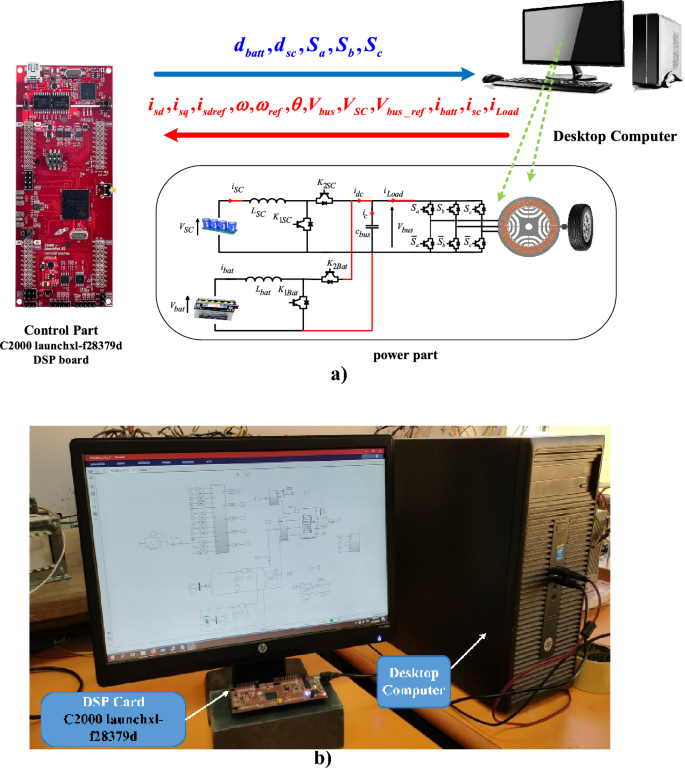
PIL co-simulation technique: (a) PIL scheme, (b) PIL platform.
After that, a configuration of the PIL process needs to be carried out primarily based on a number of line codes within the command window of the Matlab software program as follows:
Calling of the system mannequin,
Setting the com port quantity,
Defining the board charges, which characterize how briskly the pc and the DSP board will talk,
Enabling the serial communication for the PIL co-simulation,
Producing the PIL mannequin that shall be used for the PIL process.
A trial implementation in a real-time interface (RTI) using a DSpace card will be performed to reinforce the proposed power administration within the electrical automobile (EV) system. This experimental analysis goals to evaluate the efficiency of the improved power administration system.
The experimental implementation in a real-time interface (RTI) utilizing a Dspace card for the proposed power administration optimization in an electrical automobile system is a promising avenue for advancing analysis in sustainable transportation. By leveraging the computational capabilities of a Dspace card throughout the automobile’s infrastructure, the power administration system can dynamically optimize energy distribution amongst numerous elements, such because the battery, motor, and auxiliary methods, in real-time.


